!wget https://raw.githubusercontent.com/schwallergroup/ai4chem_course/generative_models/notebooks/05%20-%20Generative%20Models/utils.py -O utils.py
# download the pre-trained RNN model
!wget https://raw.githubusercontent.com/schwallergroup/ai4chem_course/generative_models/notebooks/05%20-%20Generative%20Models/data/pretrained.zinc.rnn.pth -O pretrained.rnn.pth
# download the pre-trained VAE model
!wget https://raw.githubusercontent.com/schwallergroup/ai4chem_course/generative_models/notebooks/05%20-%20Generative%20Models/data/pretrained.vae.pt -O pretrained.vae.pt
# clone RNN generative model repository
!git clone https://github.com/rociomer/dl-chem-101.git
# download the RNN training data
!wget https://raw.githubusercontent.com/schwallergroup/ai4chem_course/generative_models/notebooks/05%20-%20Generative%20Models/data/zinc.smi -O zinc.smi
# clone repository to extract the compressed molecular data
!git clone https://github.com/aksub99/molecular-vae.git
import zipfile
zip_ref = zipfile.ZipFile('molecular-vae/data/processed.zip', 'r')
zip_ref.extractall('molecular-vae/data/')
zip_ref.close()12 download a utils.py file containing some utility functions we will need
![]()
# -------------------------------------------------------------------------------------
# -------------------------------------------------------------------------------------
# -------------------------------------------------------------------------------------
# WARNING: stop here for a moment - let us know when the above cell is finished running
# -------------------------------------------------------------------------------------
# -------------------------------------------------------------------------------------
# -------------------------------------------------------------------------------------
# need to install the RNN repository as a package
%cd dl-chem-101
%cd 03_gen_SMILES_LSTM
!pip install -e .# install other packages required
!pip install rdkit
!pip install molplotly
!pip install torch
!pip install numpy
!pip install scikit-learn
!pip install h5py%cd ../..
# ***Now restart run-time of the notebook!***Week 5 Tutorial: AI for Chemistry
Molecular Generative Models
In recent years, there has been an explosion in the number of molecular generative models being developed. Regardless of the formulation, these models share some commonalities:
They can generate molecules that are not in the training data - therefore, they have the potential to explore new chemical space
They can be coupled with some optimization algorithm to explicitly tailor the model to generate molecules satisfying some target objective such as possessing high predicted solubility
You will get the chance to play with REINVENT next week which is an open-source SMILES-based generative model developed at AstraZeneca. You will get to choose what properties you want to optimize and see first-hand how the model learns to generate molecules satisfying your specified objective! 🤠 Here is an example of REINVENT in the wild - Researchers use REINVENT to design an experimentally validated nanomolar potent inhibitor
Generative models are not new and have been applied for quite some time especially in the machine learning community. Image generation is a classic example of one such application and is also what gives rise to the cool images you see generated from Stable Diffusion. Molecular generative models, however, is a less mature field that is seeing rapid progress and wide-spread adoption in industry (pharmaceutical and biotech companies).
Below are some early foundational works in the field of molecular generative models (not exhaustive): * Variational Autoencoder (VAE) this is the first example of using a VAE
Generative Adversarial Network (GAN) this is the first example of using a
GANRecurrent Neural Network (RNN) this is one of the first examples of using a
RNNRecurrent Neural Network (RNN) with Reinforcement Learning (RL): Link 1 Link 2 these are also early examples of using a
RNNbut they also coupleRLto tailor molecular generation towards desired properties
In this Part 1 Tutorial (Part 2 is next week), we introduce some of these foundational works and play around with how they generate molecules. For each generative model presented, we will provide high level details of what is going on under-the-hood and reference the original paper for details.
1. Recurrent Neural Network (RNN)
The code that is imported from utils in this section is from Rocío Mercado's dl-chem-101 repository
Note: Next week’s tutorial has 2 parts: you get to run your own REINVENT generative experiment and we break down step-by-step into exactly how REINVENT (and any SMILES-based generative model) works. For this reason, we do not show any code of the underlying model in this section
For now, a high-level summary is given.
Recurrent Neural Networks (RNN) were very popular for Natural Language Processing (NLP) (for example, machine learning on sentences to translate between languages). Generally, these models are trained to predict the next “element” (we say “element” here to be very general for this particular analogy). Consider the following sentence:
It’s so hot outside, I want to eat
based on the words seen so far, the model predicts the next “element” A reasonable next “element” would be “ice cream”, yielding the sentence:
It’s so hot outside, I want to eat ice cream
Now, let’s think about the context of this sentence. It seems reasonable to say that “ice cream” makes sense because it is hot outside. This idea of context is important for machine learning models to predict the next “element”. Unfortunately, imagine now a very long excerpt containing many paragraphs. It turns out that RNNs can struggle to “remember” long contexts. More recently, Transformers (ChatGPT is a transformer model!) have demonstrated exceptional ability to handle this problem and has now mostly replaced RNNs in NLP.
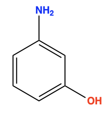
Ok, but now let’s relate what we just discussed to Molecular Generative Models. It turns out that most molecules represented as SMILES strings are not really that long and RNNs can perfectly learn to predict these relatively short SMILES sequences (compared to the example of an excerpt with many paragraphs). Correspondingly, RNN-based Molecular Generative Models have shown remarkable performance in learning the SMILES syntax. Below is an example of a molecule and its SMILES: “NC1=CC(O)=CC=C1” (not very long!)
1.1 Claim
In this section, let’s make a claim:
Training a Molecular Generative Model is not training a model to generate molecules, per say. Rather, it is to reproduce the underlying probability distribution of the training data
What does that mean? 🥴
Let’s make “predicting the next element” more concrete in the context of chemistry. SMILES-based RNNs are typically trained to predict the next token which loosely maps to individual atoms.
Let’s look at an intuitive example. Here’s Benzene:
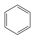
Here’s the SMILES: “c1ccccc1”
Let’s say our model is in the process of generating Benzene with this SMILES sequence so far:
“c1ccccc”
Comparing the answer, we see that we want to generate “1” This token closes the ring and recovers Benzene
Now imagine we have trained a model that can re-generate the entire dataset of SMILES. Then implicitly, the model has learned the SMILES syntax and the properties of molecules it generates overlaps with the training data. Let’s convince ourselves of this.
1.2 Is it a Molecular Generative Model or a Mime? 😵💫
Image was generated using Stable Diffusion. The prompt was “high resolution image of a mime doing chemistry”
Let’s do some exercises! We have pre-trained a generative model on a small subset of ZINC which is a database of molecules.
# loading in some helper functions (don't worry about the details here for now)
from utils import load_from_file, sample
# let's begin our dive into gaining a deeper understanding of molecular generative models
# let's load the pre-trained model
pretrained_rnn_model = load_from_file('pretrained.rnn.pth')from rdkit import Chem
# ok, let's now generate 1000 molecules from this model
# keep track of the generated molecules
generated_molecules = []
# for now, don't worry about the "sample()" and "tokenizer" code bits
# the pre-trained model provided actually does not generate valid SMILES strings every time
# we essentially keep generating until we get 1000 **valid** molecules
# NOTE: this may take a few minutes 😭
while len(generated_molecules) != 1000:
# generate token sequences
sequences, nlls = sample(model=pretrained_rnn_model)
# convert the token sequences into SMILES
smiles = pretrained_rnn_model.tokenizer.untokenize(pretrained_rnn_model.vocabulary.decode(sequences[0].numpy()))
# transform the generated SMILES into RDKit Mol objects
# the Mol object is "None" if the SMILES cannot be parted by RDKit
mol = Chem.MolFromSmiles(smiles)
if mol is not None:
# at this point, the Mol is valid so let's keep track of it
generated_molecules.append(mol)In the beginning of this notebook, we claim that all Molecular Generative Models can generate molecules that are outside the training data. Your first task is to verify this.
# there is a file called "zinc.smi" in the "data" folder that contains 50000 SMILES strings
# that form the training data for the provided pre-trained model

# with this information, your first task is to check if there is any
# overlap between the SMILES in "zinc.smi" and the generated molecules above

# Task 1: extract the SMILES from "zinc.smi"

### YOUR CODE #####
# Task 2: Get the SMILES of the generated molecules from the pre-trained model
### YOUR CODE ###### Task 3: Find out how much overlap there is between the generated SMILES
# and the training data SMILES (from "zinc.smi")
### YOUR CODE #####
# Hint: you should compare canonical SMILESThis is significant - recall in the beginning of this notebook, we said that all Molecular Generative Models can generated molecules not in the training data. You’ve just verified this! 🤩
We also said that Molecular Generative Models learn to reproduce the properties of the molecules it is trained on. ZINC actually contains a lot of "drug-like" molecules, empirically (loosely) following Lipinski's Rule of 5. "drug-likeness" can be quantified by the Quantitative Estimate of Drug-likeness (QED) score. Your next task is to verify that the QED distribution of the ZINC training data is reproduced by the pre-trained model.
# Task 4: Plot the QED score distribution of ZINC and the generated molecules
# Hint 1: RDKit has a function that computes the QED score
# Hint 2: Normalize your plot so you can see the relative distribution
#         (there are 50000 ZINC molecules compared to only 1000 generated molecules)

### YOUR CODE #####
The QED of the generated molecules overlaps with the training data! (actually the pre-trained model provided wasn’t trained to the full extent. “Proper” training of generative models will show even more significant overlap). We refer the reader to this paper - check out the figures showing overlap! You’ve now verified that Molecular Generative Models reproduce the properties of the molecules in the training data 🤩
Now let’s answer the big question from this section: Is it a Molecular Generative Model or a Mime? Let’s recap our findings:
- The model can generate
SMILESthat are not in the training data - The properties of the generated
SMILESoverlap with the training data
The answer is that Molecular Generative Models are kind of like a mime. You can generate new molecules that fit into the properties distribution in your training data. When could this be useful? Imagine you have a dataset of molecules with properties in the range that you are interested in. The out-of-the-box Molecular Generative Models can give you new molecules within this properties range! What if you want to generate molecules outside the training data properties distribution? Turns out what we presented here is the foundation for coupling optimization algorithms which can shift the probability distribution of the Molecular Generative Model to the property ranges you want. Next week, you will see this first-hand with a practical tutorial on REINVENT.
Finally, let’s just take a look at some of the generated molecules.
# Task 5: Visually inspect a few of the generated molecules

### YOUR CODE ###
Let’s now show another Molecular Generative Model class.
2. Variational Autoencoder (VAE)
Image was generated using Stable Diffusion. The prompt was “a chef flattens a pancake”
What do pancakes have to do with VAEs? (but also let me know where the best pancakes in Lausanne are 🥞) In this section, we present a high-level overview of what VAEs do. Imagine you have a stack of pancakes, some with blueberries and some with raspberries. You then take the biggest spatula you can find and squash it such that you can’t even distinguish the pancakes from each other anymore - they are all combined together into a giant pancake like in the image. Now imagine the surface of this giant flat pancake. You start looking around and you notice some blueberries and think to yourself, “this must have came from the blueberry pancake originally”. You look around some more and you see another piece of pancake but with both blueberries and raspberries. There were no original pancakes with both berries so you conclude that this piece of pancake must have been from a little bit of the blueberry pancake and a little bit of the raspberry pancake.
Remembering this analogy, we now present a high-level overview of VAEs starting with a classic image of the model. This particular image is from Saul Dobilas.
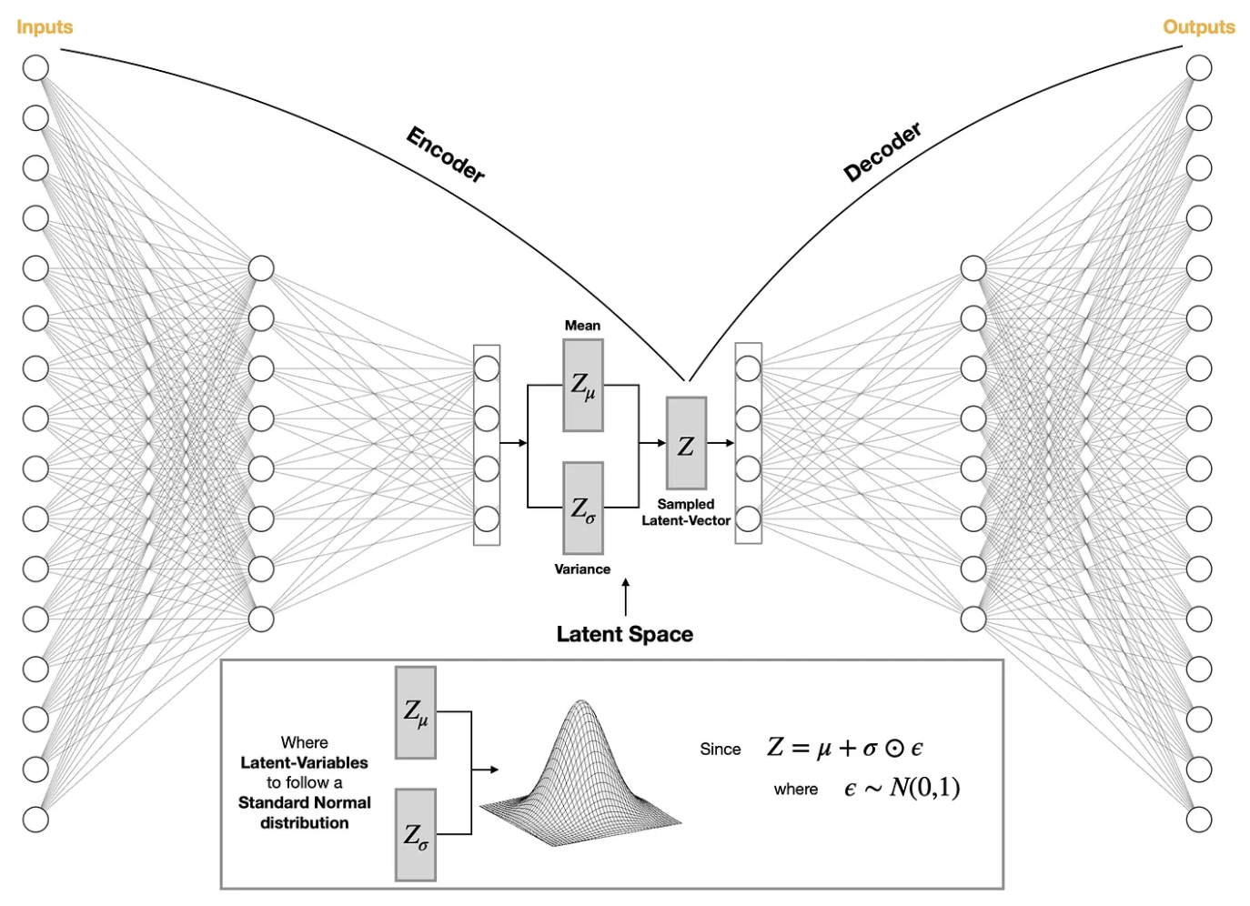
The Encoder takes molecules and converts it into a low-dimensional vector and maps it onto a Gaussian Distribution. Recall that Gaussian Distributions are completely defined by their mean and variance. Specifically, knowing both the mean and variance allows you to construct the full Gaussian Distribution. The Latent Vector is now computed based on the mean and variance but with some noise added to it. In the image, this noise is drawn from a Gaussian Distribution. The job of the Decoder is to take this Latent Vector and reconstruct the input.
Let’s tie this back to the pancakes analogy. By converting all molecules into a low-dimensional vector via the Encoder, a continuous Latent Space is created. We squash all our blueberry and raspberry pancakes into a single giant pancake (we take all our molecules and “flatten” them). The model can be trained to reconstruct the blueberry pancake (some molecule) given the squashed blueberry pancake (the Latent Vector). What happens when you get to the pancake piece that has both blueberries and raspberries? By defining a continuous Latent Space, the reconstructed molecule from this chunk of pancake is a hybrid between blueberry and raspberry. This is where the Generative Molecular Model comes in: by sampling Latent Vectors from the Latent Space, the Decoder can reconstruct different molecules back!
In the original molecular VAE paper, they train a neural network model to predict properties in the Latent Space. They also show how you can move in the Latent Space to go from some starting molecule to another molecules with desired properties. Here, we omit further details and instead try to visually demonstrate what the Latent Space is.
Note: The VAE code from this section is taken from Akshay Subramanian who reimplemented the original VAE in PyTorch in this Jupyter notebook
The code is shown here but you do not have to go over anything/everything. It is shown here to highlight the key steps that occur. Some comments have been added to map the big idea of what is happening back to the VAE image above.
Further Note: There are no tasks in this section
# imports
import torch
import torch.nn as nn
import torch.nn.functional as F
import torch.utils.data
import gzip
import pandas
import h5py
import numpy as np
from __future__ import print_function
import argparse
import os
import h5py
import torch.optim as optim
from torch.optim.lr_scheduler import ReduceLROnPlateau
from sklearn import model_selection
# these are utility functions
def one_hot_array(i, n):
return map(int, [ix == i for ix in xrange(n)])
def one_hot_index(vec, charset):
return map(charset.index, vec)
def from_one_hot_array(vec):
oh = np.where(vec == 1)
if oh[0].shape == (0, ):
return None
return int(oh[0][0])
def decode_smiles_from_indexes(vec, charset):
return b"".join(map(lambda x: charset[x], vec)).strip()
def load_dataset(filename, split = True):
h5f = h5py.File(filename, 'r')
if split:
data_train = h5f['data_train'][:]
else:
data_train = None
data_test = h5f['data_test'][:]
charset = h5f['charset'][:]
h5f.close()
if split:
return (data_train, data_test, charset)
else:
return (data_test, charset)# the main code for the VAE
class MolecularVAE(nn.Module):
def __init__(self):
super().__init__()
# encoder related blocks
self.conv_1 = nn.Conv1d(120, 9, kernel_size=9)
self.conv_2 = nn.Conv1d(9, 9, kernel_size=9)
self.conv_3 = nn.Conv1d(9, 10, kernel_size=11)
self.linear_0 = nn.Linear(70, 435)
self.linear_1 = nn.Linear(435, 292)
self.linear_2 = nn.Linear(435, 292)
# decoder related blocks
self.linear_3 = nn.Linear(292, 292)
self.gru = nn.GRU(292, 501, 3, batch_first=True)
self.linear_4 = nn.Linear(501, 33)
# activation function
self.relu = nn.ReLU()
def encode(self, x):
# forward pass through encoder (pancake squashing!)
x = self.relu(self.conv_1(x))
x = self.relu(self.conv_2(x))
x = self.relu(self.conv_3(x))
x = x.view(x.size(0), -1)
x = F.selu(self.linear_0(x))
return self.linear_1(x), self.linear_2(x)
def sampling(self, z_mean, z_logvar):
# recall in the VAE figure, noise is added
# epsilon is the noise
epsilon = 1e-2 * torch.randn_like(z_logvar)
# return the latent vector (this is what the decoder will use to reconstruct the input)
return torch.exp(0.5 * z_logvar) * epsilon + z_mean
def decode(self, z):
# forward pass through decoder to go from latent vector back to a molecule
z = F.selu(self.linear_3(z))
z = z.view(z.size(0), 1, z.size(-1)).repeat(1, 120, 1)
output, hn = self.gru(z)
out_reshape = output.contiguous().view(-1, output.size(-1))
y0 = F.softmax(self.linear_4(out_reshape), dim=1)
y = y0.contiguous().view(output.size(0), -1, y0.size(-1))
return y
def forward(self, x):
# the overall forward pass takes the input, passes it to the encoder and then decoder
# first encode your input to get the mean and variance of the Gaussian distribution it is mapped to
z_mean, z_logvar = self.encode(x)
# get the latent vector taking the mean and variance above and adding noise t it
z = self.sampling(z_mean, z_logvar)
# decode the latent vector, z, to reconstruct a molecule
return self.decode(z), z_mean, z_logvar
def vae_loss(x_decoded_mean, x, z_mean, z_logvar):
# the loss function is a combination of 2 quantities:
# 1. "reconstruction loss" which measures how different the reconstructed molecule
# is to the original. We would want them to be similar
# 2. "Kullback–Leibler (KL) divergence". We are trying to approximate the distribution
# of the latent vector with a Gaussian distribution. The KL divergence measure how "off" we are
reconstruction_loss = F.binary_cross_entropy(x_decoded_mean, x, size_average=False)
kl_loss = -0.5 * torch.sum(1 + z_logvar - z_mean.pow(2) - z_logvar.exp())
return reconstruction_loss + kl_loss# this was used when we pre-trained the VAE
# it initializes a PyTorch DataLoader so we can read batches of molecules at a time during training
data_train, data_test, charset = load_dataset('molecular-vae/data/processed.h5')
data_train = torch.utils.data.TensorDataset(torch.from_numpy(data_train))
train_loader = torch.utils.data.DataLoader(data_train, batch_size=500, shuffle=True)# initiate an instance of the MolecularVAE
pretrained_vae = MolecularVAE()
# load the pre-trained model (we provide this)
pretrained_vae.load_state_dict(torch.load('pretrained.vae.pt'))Starting below, we will visualize the Latent Space.
# RERUN HERE FOR NEW MOLECULES!
# this bit of code randomly takes 500 molecules from the training data
for batch in train_loader:
    training_data_molecules = batch
# manually add some noise to the training data molecules --> we will see
# what these "noised" molecules look like in the latent space later
num_noised = 10
noised_molecules = training_data_molecules[0][:num_noised] + torch.normal(0, 0.0001, (num_noised, 120, len(charset)))# this bit of code gets the SMILES back from the 500 training data molecules we got above
smiles_list = []
for idx in range(training_data_molecules[0].shape[0]):
vector = training_data_molecules[0][idx].reshape(1, 120, len(charset)).argmax(axis=2)[0]
smiles = decode_smiles_from_indexes(vector, charset)
smiles = str(smiles).replace("'", '').replace('b', '')
smiles_list.append(smiles)# this bit of code gets the SMILES from the "noised" training data molecules
noised_smiles_list = []
for idx in range(noised_molecules.shape[0]):
vector = noised_molecules[idx].reshape(1, 120, len(charset)).argmax(axis=2)[0]
smiles = decode_smiles_from_indexes(vector, charset)
smiles = str(smiles).replace("'", '').replace('b', '')
noised_smiles_list.append(smiles)# encode the training data SMILES
z_mean, z_logvar = pretrained_vae.encode(training_data_molecules[0])
# get the latent space
latent_space = pretrained_vae.sampling(z_mean, z_logvar)
# encode the noised data
noised_z_mean, noised_z_logvar = pretrained_vae.encode(noised_molecules)
# get the latent space of the "noised" molecules
noised_latent_space = pretrained_vae.sampling(noised_z_mean, noised_z_logvar)# the code here plots an interative latent space - hover around the space and explore the molecules!
import plotly
import plotly.express as px
import molplotly
import pandas as pd
all_smiles = smiles_list + noised_smiles_list
full_latent_space = torch.vstack([latent_space, noised_latent_space])
plotting_df = pd.DataFrame({'smiles': all_smiles,
'group': ['Training Data']*500 + ['Sampled from Latent Space']*num_noised,
'latent_space_x': full_latent_space[:, 0].detach(),
'latent_space_y': full_latent_space[:, 1].detach()})
fig_scatter = px.scatter(plotting_df,
x='latent_space_x',
y='latent_space_y',
color='group')
app_scatter = molplotly.add_molecules(fig=fig_scatter,
df=plotting_df,
smiles_col='smiles',
title_col='group',
color_col='group')
app_scatter.run_server(mode='inline', height=400)
# the red points are the "sampled" molecules created from adding "noise" to the latent vectors of the
# training data molecules. Here, let's bring back the analogy of the blueberry and raspberry pancakes.
# Locate a red point and look at the training data points around it. You should be able to see some
# structural similarities. One can think of the red point as a "hybrid" between its surrounding neighbours
# of blue points, i.e., it's a hybrid between blueberry and raspberry
# Note: it could be that sometimes "close" points are not that similar - this has to do with the "smoothness"
# of the latent space such that there are abrupt changes
# Finally, if you want to see new molecules, re-run the cell above marked with "RERUN HERE FOR NEW MOLECULES!"